5. Model Metrics¶

Evaluating your machine learning algorithm is an essential. Your model may give you satisfying results when evaluated using a metric say accuracy_score but may give poor results when evaluated against other metrics such as logarithmic_loss or any other such metric. Most of the times we use classification accuracy to measure the performance of our model, however it is not enough to truly judge our model. Different performance metrics are used to evaluate different Machine Learning Algorithms. We can use classification performance metrics such as Log-Loss, Accuracy, AUC(Area under Curve) etc. Another example of metric for evaluation of machine learning algorithms is precision, recall, which can be used for sorting algorithms primarily used by search engines.

The metrics that you choose to evaluate your machine learning model is very important. Choice of metrics influences how the performance of machine learning algorithms is measured and compared.

5.1. Mean Absolute Error¶

Mean Absolute Error(MAE) is the average of the difference between the Original Values and the Predicted Values. It gives us the measure of how far the predictions were from the actual output. However, they don’t gives us any idea of the direction of the error i.e. whether we are under predicting the data or over predicting the data.

If \(\hat{y_i}\) is the predicted value of the \(i^{th}\) sample, and \(y_i\) is the corresponding true value, then the mean absolute error (MAE) estimated over \(n_{\text{samples}}\) is defined as:

(1)¶\[\text{MAE}(y, \hat{y}) = \frac{1}{n_{\text{samples}}} \sum_{i=0}^{n_{\text{samples}}-1} \left| y_i - \hat{y}_i \right|\]

5.2. Mean Squared Error¶

Mean Squared Error(MSE) is quite similar to Mean Absolute Error, the only difference being that MSE takes the average of the square of the difference between the original values and the predicted values. The advantage of MSE being that it is easier to compute the gradient, whereas Mean Absolute Error requires complicated linear programming tools to compute the gradient. As, we take square of the error, the effect of larger errors become more pronounced then smaller error, hence the model can now focus more on the larger errors.

If \(\hat{y_i}\) is the predicted value of the \(i^{th}\) sample, and \(y_i\) is the corresponding true value, then the mean absolute error (MAE) estimated over \(n_{\text{samples}}\) is defined as:

(2)¶\[\text{MSE}(y, \hat{y}) = \frac{1}{n_\text{samples}} \sum_{i=0}^{n_\text{samples} - 1} (y_i - \hat{y}_i)^2\]

5.3. Log Loss¶

Log loss, also called logistic regression loss or cross-entropy loss, is defined on probability estimates. It is commonly used in (multinomial) logistic regression and neural networks, as well as in some variants of expectation-maximization, and can be used to evaluate the probability outputs of a model instead of its discrete predictions.

5.3.1. Binary Classification¶

For binary classification with a true label \(y \in \{0,1\}\) and a probability estimate \(p = \operatorname{Pr}(y = 1)\), the log loss per sample is the negative log-likelihood of the classifier given the true label:

(3)¶\[L_{\log}(y, p) = -\log \operatorname{Pr}(y|p) = -(y \log (p) + (1 - y) \log (1 - p))\]

5.3.2. Multiclass Classification¶

Let the true labels for a set of samples be encoded as a 1-of-K binary indicator matrix \(Y\), i.e., \(y_{i,k} = 1\) if sample \(i\) has label \(k\) taken from a set of \(K\) labels. Let \(P\) be a matrix of probability estimates, with \(p_{i,k} = \operatorname{Pr}(t_{i,k} = 1)\). Then the log loss of the whole set is:

(4)¶\[L_{\log}(Y, P) = -\log \operatorname{Pr}(Y|P) = - \frac{1}{N} \sum_{i=0}^{N-1} \sum_{k=0}^{K-1} y_{i,k} \log p_{i,k}\]

where,

\(y_{i,k}\), indicates whether sample \(i\) belongs to class \(k\) or not
\(p_{i,k}\), indicates the probability of sample \(i\) belonging to class \(j\)

Note

To see how this generalizes the binary log loss given above, note that in the binary case, \(p_{i,0} = 1 - p_{i,1}\) and \(y_{i,0} = 1 - y_{i,1}\), so expanding the inner sum over \(y_{i,k} \in \{0,1\}\) gives the binary log loss. Log Loss has no upper bound and it exists on the range \([0, \infty)\). Log Loss nearer to \(0\) indicates higher accuracy, whereas if the Log Loss is away from \(0\) then it indicates lower accuracy. In general, minimizing Log Loss gives greater accuracy for the classifier.

In simpler terms, Log Loss works by penalizing the false classifications. It works well for multi-class classification.

5.4. Confusion Matrix¶

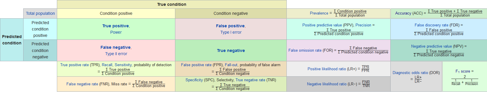
The Confusion matrix is one of the most intuitive and easiest metric used for finding the correctness and accuracy of the model. It is used for Classification problem where the output can be of two or more types of classes. It in itself is not a performance measure as such, but almost all of the performance metrics are based on Confusion Matrix.

Lets say we have a classification problem where we are predicting if a person has cancer or not.

P : a person tests positive for cancer
N : a person tests negative for cancer

The confusion matrix, is a table with two dimensions (“Actual” and “Predicted”), and sets of “classes” in both dimensions. Our Actual classifications are rows and Predicted ones are Columns.

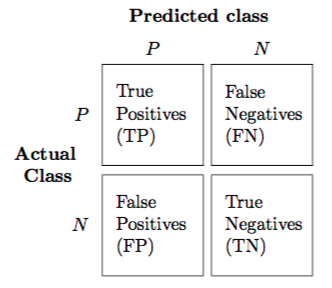
5.4.1. Key Terms¶

True Positives (TP):
- True positives are the cases when the actual class of the data point was Positive and the predicted is also Positive. Ex: The case where a person is actually having cancer (Positive) and the model classifying his case as cancer (Positive) comes under True positive.
True Negatives (TN):
- True negatives are the cases when the actual class of the data point was Negative and the predicted is also Negative. Ex: The case where a person NOT having cancer and the model classifying his case as Not cancer comes under True Negatives.
False Positives (FP):
- False positives are the cases when the actual class of the data point was Negative and the predicted is Positive. False is because the model has predicted incorrectly and positive because the class predicted was a positive one. (Positive). Ex: A person NOT having cancer and the model classifying his case as cancer comes under False Positives.
False Negatives (FN):
- False negatives are the cases when the actual class of the data point was Positive (True) and the predicted is Negative. False is because the model has predicted incorrectly and negative because the class predicted was a negative one. (Negative). Ex: A person having cancer and the model classifying his case as No-cancer comes under False Negatives.

5.5. Classification Accuracy¶

Classification Accuracy is what we usually mean, when we use the term accuracy. If \(\hat{y}_i\) is the predicted value of the \(i^{th}\) sample and \(y_i\) is the corresponding true value, then the fraction of correct predictions over \(n_\text{samples}\) is defined as:

(5)¶\[\texttt{accuracy}(y, \hat{y}) = \frac{1}{n_\text{samples}} \sum_{i=0}^{n_\text{samples}-1} 1(\hat{y}_i = y_i)\]

In short, it is the ratio of number of correct predictions to the total number of input samples:

(6)¶\[\text{accuracy} = \frac{\text{Number of Correct Predictions}}{\text{Total Number of Predictions made}} = \frac{\text{TP + TN}}{\text{TP+TN+FP+FN}}\]

Accuracy is a good measure when the target variable classes in the data are nearly balanced. Ex: 60% classes in our fruits images data are apple and 40% are oranges. A model which predicts whether a new image is Apple or an Orange, 97% of times correctly is a very good measure in this example.
Accuracy should NEVER be used as a measure when the target variable classes in the data are a majority of one class. Ex: In a cancer detection example with 100 people, only 5 people has cancer. Let’s say our model is very bad and predicts every case as No Cancer. In doing so, it has classified those 95 non-cancer patients correctly and 5 cancerous patients as Non-cancerous. Now even though the model is terrible at predicting cancer, The accuracy of such a bad model is also 95%.

5.6. Precision¶

Using our cancer detection example, Precision is a measure that tells us what proportion of patients that we diagnosed as having cancer, actually had cancer. The predicted positives (People predicted as cancerous are TP and FP) and the people actually having a cancer are TP.

(7)¶\[\text{Precision} = \frac{\text{TP}}{\text{TP+FP}}\]

Ex: In our cancer example with 100 people, only 5 people have cancer. Let’s say our model is very bad and predicts every case as Cancer. Since we are predicting everyone as having cancer, our denominator(True positives and False Positives) is 100 and the numerator, person having cancer and the model predicting his case as cancer is 5. So in this example, we can say that Precision of such model is 5%.

5.7. Recall or Sensitivity¶

Recall is a measure that tells us what proportion of patients that actually had cancer was diagnosed by the algorithm as having cancer. The actual positives (People having cancer are TP and FN) and the people diagnosed by the model having a cancer are TP. (Note: FN is included because the Person actually had a cancer even though the model predicted otherwise).

(8)¶\[\text{Recall} = \frac{\text{TP}}{\text{TP+FN}}\]

Ex: In our cancer example with 100 people, 5 people actually have cancer. Let’s say that the model predicts every case as cancer. So our denominator(True positives and False Negatives) is 5 and the numerator, person having cancer and the model predicting his case as cancer is also 5(Since we predicted 5 cancer cases correctly). So in this example, we can say that the Recall of such model is 100%. And Precision of such a model(As we saw above) is 5%.

Precision is about being precise. So even if we managed to capture only one cancer case, and we captured it correctly, then we are 100% precise.
Recall is not so much about capturing cases correctly but more about capturing all cases that have “cancer” with the answer as “cancer”. So if we simply always say every case as “cancer”, we have 100% recall.

5.8. F1 Score¶

F1 Score, also known as the Sørensen–Dice coefficient or Dice similarity coefficient(DSC), is the Harmonic Mean between precision and recall. The range for F1 Score is [0, 1]. It tells you how precise your classifier is (how many instances it classifies correctly), as well as how robust it is (it does not miss a significant number of instances).

High precision but lower recall, gives you an extremely accurate, but it then misses a large number of instances that are difficult to classify. The greater the F1 Score, the better is the performance of our model.

(9)¶\[{\displaystyle F_{1}=\left({\frac {\mathrm {recall} ^{-1}+\mathrm {precision} ^{-1}}{2}}\right)^{-1}=2\cdot {\frac {\mathrm {precision} \cdot \mathrm {recall} }{\mathrm {precision} +\mathrm {recall} }}}\]

Two other commonly used F measures are the \(F_{2}\) measure, which weighs recall higher than precision (by placing more emphasis on false negatives), and the \(F_{0.5}\) measure, which weighs recall lower than precision (by attenuating the influence of false negatives).

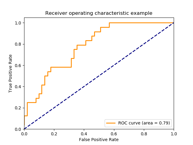
5.9. Receiver operating characteristic (ROC)¶

Receiver operating characteristic (ROC), or simply ROC curve, is a graphical plot which illustrates the performance of a binary classifier system as its discrimination threshold is varied. It is created by plotting the fraction of true positives out of the positives (TPR = true positive rate) vs. the fraction of false positives out of the negatives (FPR = false positive rate), at various threshold settings. TPR is also known as sensitivity, and FPR is one minus the specificity or true negative rate.

5.9.1. True Positive Rate (Sensitivity)¶

True Positive Rate corresponds to the proportion of positive data points that are correctly considered as positive, with respect to all positive data points.

(10)¶\[\text{TruePositiveRate} = \frac{\text{True Positive}}{\text{True Positive + False Negative}}\]

5.9.2. False Positive Rate (Specificity)¶

False Positive Rate corresponds to the proportion of negative data points that are mistakenly considered as positive, with respect to all negative data points.

(11)¶\[\text{FalsePositiveRate} = \frac{\text{False Positive}}{\text{False Positive + True Negative}}\]

This function requires the true binary value and the target scores, which can either be probability estimates of the positive class, confidence values, or binary decisions. False Positive Rate and True Positive Rate both have values in the range [0, 1]. FPR and TPR both are computed at threshold values such as (0.00, 0.02, 0.04, …., 1.00) and a graph is drawn.

Lowering the classification threshold classifies more items as positive, thus increasing both False Positives and True Positives. To compute the points in an ROC curve, we could evaluate a logistic regression model many times with different classification thresholds.

5.10. AUC: Area Under the ROC Curve¶

Area under the ROC Curve, is the measure of an entire two-dimensional area underneath the entire ROC curve (think integral calculus) from (0,0) to (1,1). AUC provides an aggregate measure of performance across all possible classification thresholds. AUC ranges in value from 0 to 1. A model whose predictions are 100% wrong has an AUC of 0.0; one whose predictions are 100% correct has an AUC of 1.0.

One way of interpreting AUC is as the probability that the model ranks a random positive example more highly than a random negative example. Ex: given the following examples, which are arranged from left to right in ascending order of logistic regression predictions; AUC represents the probability that a random positive (green) example is positioned to the right of a random negative (red).

5.10.1. Properties¶

AUC is scale-invariant. It measures how well predictions are ranked, rather than their absolute values.
AUC is classification-threshold-invariant. It measures the quality of the model’s predictions irrespective of what classification threshold is chosen.
Scale invariance is not always desirable. For example, sometimes we really do need well calibrated probability outputs, and AUC won’t tell us about that.
Classification-threshold invariance is not always desirable. In cases where there are wide disparities in the cost of false negatives vs. false positives, it may be critical to minimize one type of classification error. AUC isn’t a useful metric for this type of optimization.

Citations

Footnotes

References