3. Bias and Variance
3.1. Bias
It is the difference between the average prediction of our model and the correct value which we are trying to predict. Model with high bias pays very little attention to the training data and oversimplifies the model. It always leads to high error on training and test data.
3.2. Variance
It is the variability of model prediction for a given data point or a value which tells us spread of our data. Model with high variance pays a lot of attention to training data and does not generalize on the data which it hasn’t seen before. As a result, such models perform very well on training data but has high error rates on test data.
3.3. Differences
- Bias is the algorithm’s tendency to consistently learn the wrong thing by not taking into account all the information in the data (underfitting). Variance is the algorithm’s tendency to learn random things irrespective of the real signal by fitting highly flexible models that follow the error/noise in the data too closely (overfitting).
- Bias is also used to denote by how much the average accuracy of the algorithm changes as input/training data changes. Similarly, Variance is used to denote how sensitive the algorithm is to the chosen input data. Bias is prejudice in favor of or against one thing, person, or group compared with another, usually in a way considered to be unfair. Variance is the state or fact of disagreeing or quarreling.
3.4. Mathematical Representation
Let the variable we are trying to predict as \(y\) and other covariates as \(x\). We assume there is a relationship between the two such that
The expected squared error at a point \(x\) is:
The \(Err(x)\) can be further decomposed as :
where
- \(e\) is the error term and it’s normally distributed with a mean of 0.
- \(f\) = Target function
- \(\hat{f}\) = estimation of Target function
3.4.1. Irreducible error
The above error can’t be reduced by creating good models. It is a measure of the amount of noise in our data. Here it is important to understand that no matter how good we make our model, our data will have certain amount of noise or irreducible error that can not be removed.
3.4.2. Bias error
The above equation is little confusing because we can learn only one estimate for the target function \(\hat{f}\) using the data we sampled, but the above equation takes expectation for \(\hat{f}\). Assume that we sampled a data for \(n\) times and make a model for each sampled data. We can’t expect same data every time due to irreducible error influence in the target function. As the data changes every time, our estimation of target function also change every time.
Note
Bias will be zero if, \(E[\hat{f}(x)] = f(x)\). This is not possible if we make assumptions to learn the target function.
Most of the parametric methods make assumption(s) to learn a target function. The methods which make more assumptions to learn a target function are high biased method. Similarly, the methods which make very less assumptions to learn a target function are low biased method.
- Examples of low-bias machine learning algorithms: Decision Trees, k-Nearest Neighbors and Support Vector Machines.
- Examples of high-bias machine learning algorithms: Linear Regression, Linear Discriminant Analysis and Logistic Regression
3.4.3. Variance error
As mentioned before, for different data set, we will get different estimation for the target function. The variance error measure how much our target function \((\hat{f})\) would differ if a new training data was used. For example, let the target fucntion be given as \(f=\beta_0 + \beta_1 ∗ X\) ; if we use regression method to learn the given target function and assume the same functional form to estimate the target function, then the number of possible estimated function will be limited. Even though we get different \((\hat{f})\) for different training data, our search space is limited due to functional form.
Note
If we use K-Nearest Neighbor algorithm, KNN algorithm search the estimation for target function in large dimensional space.
- If we sample different training data for the same variables and the estimated function suggests small changes from the previous \((\hat{f})\) , then our model is low variance one.
- If we sample different training data for the same variables and the estimated function suggests large changes from the previous \((\hat{f})\) , then our model is high variance one.
3.5. Bias-Variance Tradeoff
If our model is too simple and has very few parameters then it may have high bias and low variance. On the other hand if our model has large number of parameters then it’s going to have high variance and low bias. So we need to find the right/good balance without overfitting and underfitting the data. This tradeoff in complexity is why there is a tradeoff between bias and variance. An algorithm can’t be more complex and less complex at the same time.
At its root, dealing with bias and variance is really about dealing with over- and under-fitting. Bias is reduced and variance is increased in relation to model complexity. As more and more parameters are added to a model, the complexity of the model rises and variance becomes our primary concern while bias steadily falls. For example, as more polynomial terms are added to a linear regression, the greater the resulting model’s complexity will be. In other words, bias has a negative first-order derivative in response to model complexity while variance has a positive slope.
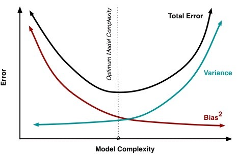
Understanding bias and variance is critical for understanding the behavior of prediction models, but in general what you really care about is overall error, not the specific decomposition. The sweet spot for any model is the level of complexity at which the increase in bias is equivalent to the reduction in variance.
If our model complexity exceeds this sweet spot, we are in effect over-fitting our model; while if our complexity falls short of the sweet spot, we are under-fitting the model. In practice, there is not an analytical way to find this location. Instead we must use an accurate measure of prediction error and explore differing levels of model complexity and then choose the complexity level that minimizes the overall error. A key to this process is the selection of an accurate error measure as often grossly inaccurate measures are used which can be deceptive.
Citations
Footnotes
References