2. Simple Linear Regression
Linear regression is an approach for predicting a quantitative response using feature predictor or input variable. It is a basic predictive analytics technique that uses historical data to predict an output variable. It takes the following form:
where,
- \(y\) is the response, a function of x
- \(x\) is the feature
- \(beta_{0}\) is the intercept, also called bias coefficient
- \(beta_{1}\) is the slope, also called the scale factor
- \(beta_{0}\) and \(\beta_{1}\) are called the model coefficients
Our goal is to find statistically significant values of the parameters \(\beta_0\) and \(\beta_1\) that minimize the difference between \(y\) ( output ) and \(y_e\) ( estimated / predicted output ).
Note
The predicted values here are continuous in nature. So, your ultimate goal is, given a training set, to learn a function \(f:X→Y\) so that \(f(x)\) is a good predictor for the corresponding value of \(y\). Also, keep in mind that the domain of values both \(x\) and \(y\) are all real numbers
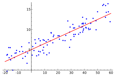
If we are able to determine the optimum values of these two parameters, then we will have the Line of Best Fit that we can use to predict the values of \(y\), given the value of \(x\).
It is important to note that, linear regression can often be divided into two basic forms:
- Simple Linear Regression (SLR) which deals with just two variables (the one you saw at first)
- Multi-linear Regression (MLR) which deals with more than two variables
So, how do we estimate \(\beta_{0}\) and \(\beta_{1}\)? We can use a method called ordinary least squares.
2.1. Ordinary Least Sqaure
2.1.1. Method
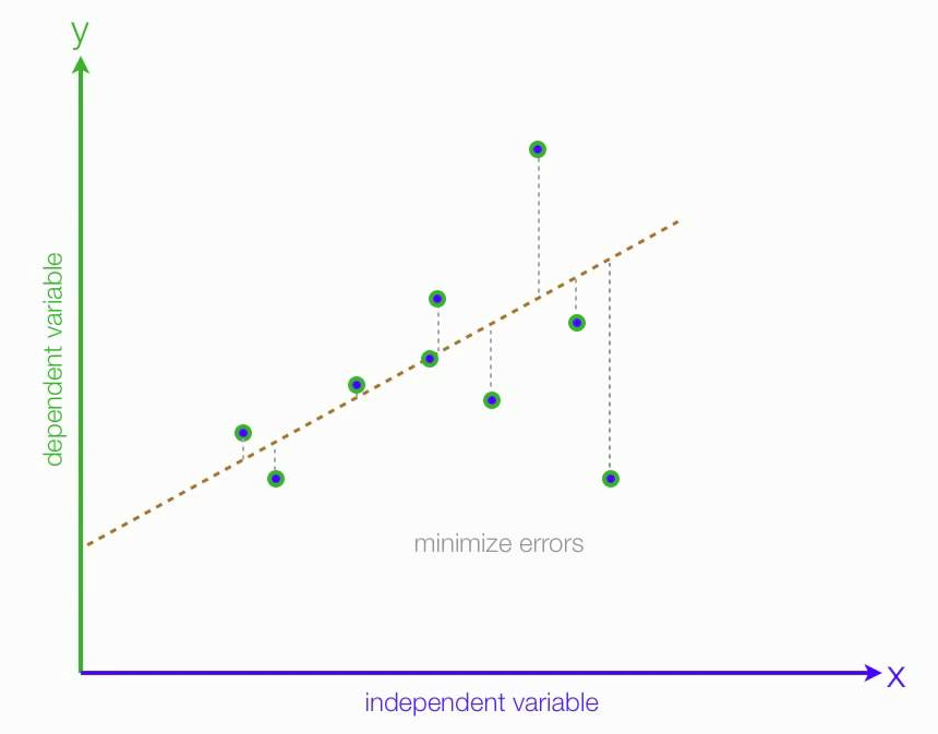
Ordinary least squares (OLS) is a type of linear least squares method for estimating the unknown parameters in a linear regression model. OLS chooses the parameters of a linear function of a set of explanatory variables by the principle of least squares: minimizing the sum of the squares of the differences between the observed dependent variable (values of the variable being predicted) in the given dataset and those predicted by the linear function.
This is seen as the sum of the squared distances, parallel to the axis of the dependent variable, between each data point in the set and the corresponding point on the regression surface – the smaller the differences, the better the model fits the data.
The least squares estimates in this case are given by simple formulas:
where,
- Var(.) and Cov(.) are called sample parameters.
- \(\beta_{1}\) is the slope
- \(\beta_{0}\) is the intercept
2.1.2. Evaluation
There are many methods to evaluate models. We will use Root Mean Squared Error and Coefficient of Determination
Root Mean Squared Error is the square root of sum of all errors divided by number of values:
(2)¶\[RMSE = \sqrt{\sum_{i=1}^{n}{\frac{1}{n}(\hat{y_{i}}-{y_i})^2}}\]R^2 Error score usually range from 0 to 1. It will also become negative if the model is completely wrong:
(3)¶\[\begin{split}\operatorname{R^2}&=1-\frac{\text{Total Sum of Squares}}{\text{Total Sum of Square of Residuals}} \\ &=1-\frac{\sum_{i=1}^{n}(y_{i}-\hat{y_{i}})^2}{\sum_{i=1}^{n}(y_{i}-\bar{y})^2}\end{split}\]
Note
We want to minimize the error of our model. A good model will always have least error. We can find this line by reducing the error. The error of each point is the distance between line and that point as illustrated as above
Citations
Footnotes
References