8. Gradient descent

Gradient Descent is a method used while training a machine learning model. It is an optimization algorithm, based on a convex function, that tweaks it’s parameters iteratively to minimize a given function to its local minimum. It is simply used to find the values of a functions parameters (coefficients) that minimize a cost function as far as possible. You start by defining the initial parameters values and from there on Gradient Descent iteratively adjusts the values, using calculus, so that they minimize the given cost-function

8.1. Gradient

A gradient measures how much the output of a function changes if you change the inputs a little bit. It simply measures the change in all weights with regard to the change in error. You can also think of a gradient as the slope of a function. The higher the gradient, the steeper the slope and the faster a model can learn. But if the slope is zero, the model stops learning. Said it more mathematically, a gradient is a partial derivative with respect to its inputs.

8.2. Cost Function

It is a way to determine how well the machine learning model has performed given the different values of each parameters. The linear regression model, the parameters will be the two coefficients, \(\beta\) and \(m\) :

\[y = \beta + mx_{1}\]

The cost function will be the sum of least square methods. Since the cost function is a function of the parameters \(\beta\) and \(m\), we can plot out the cost function with each value of the coefficients. (i.e. Given the value of each coefficient, we can refer to the cost function to know how well the machine learning model has performed). The cost function looks like:

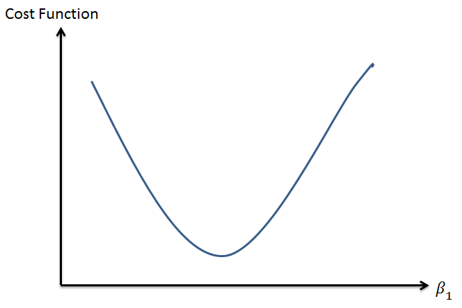
1. during the training phase, we are focused on selecting the ‘best’ value for the parameters (i.e. the coefficients), \(x\)’s will remain the same throughout the training phase
2. for the case of linear regression, we are finding the value of the coefficients that will reduce the cost to the minimum a.k.a the lowest point in the mountainous region.

8.3. Method

The Cost function will take in a \((m,b)\) pair and return an error value based on how well the line fits our data. To compute this error for a given line, we’ll iterate through each \((x,y)\) point in our data set and sum the square distances between each point’s \(y\) value and the candidate line’s \(y\) value (computed at mx + b). It’s conventional to square this distance to ensure that it is positive and to make our error function differentiable.

• Lines that fit our data better (where better is defined by our error function) will result in lower error values. If we minimize this function, we will get the best line for our data. Since our error function consists of two parameters (m and b) we can visualize it as a two-dimensional surface.

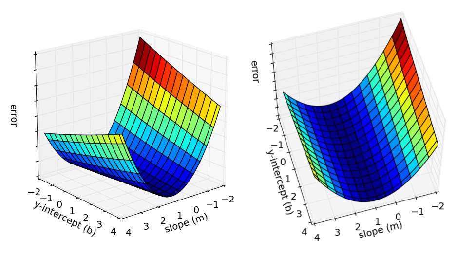
• Each point in this two-dimensional space represents a line. The height of the function at each point is the error value for that line. Some lines yield smaller error values than others (i.e., fit our data better). When we run gradient descent search, we will start from some location on this surface and move downhill to find the line with the lowest error.

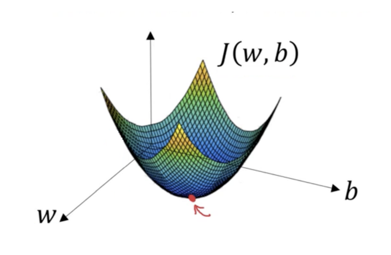
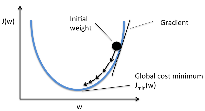
• The horizontal axes represent the parameters (\(w\) and \(\beta\)) and the cost function \(J(w, \beta)\) is represented on the vertical axes. You can also see in the image that gradient descent is a convex function.
• we want to find the values of \(w\) and \(\beta\) that correspond to the minimum of the cost function (marked with the red arrow). To start with finding the right values we initialize the values of \(w\) and \(\beta\) with some random numbers and Gradient Descent then starts at that point.
• Then it takes one step after another in the steepest downside direction till it reaches the point where the cost function is as small as possible.

8.4. Algorithm

Moving forward to find the lowest error (deepest valley) in the cost function (with respect to one weight) we need to tweak the parameters of the model. Using calculus, we know that the slope of a function is the derivative of the function with respect to a value. This slope always points to the nearest valley.

(1)\[Error_{(m,\beta)} = \frac{1}{N}\sum_{i=1}^{N}(y_{i}-(mx_{i} + \beta))^2\]

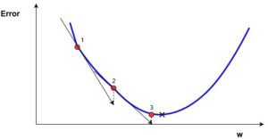
We can see the graph of the cost function(named \(Error\) with symbol \(J\)) against just one weight. Now if we calculate the slope(let’s call this \((\frac{dJ}{dw})\) of the cost function with respect to this one weight, we get the direction we need to move towards, in order to reach the local minima(nearest deepest valley).

Note

The gradient (or derivative) tells us the incline or slope of the cost function. Hence, to minimize the cost function, we move in the direction opposite to the gradient.

8.4.1. Steps

1. Initialize the weights \(w\) randomly.
2. Calculate the gradients \(G\) of cost function w.r.t parameters. This is done using partial differentiation: \(G = ∂J(w)/∂w\). The value of the gradient \(G\) depends on the inputs, the current values of the model parameters, and the cost function.
3. Update the weights by an amount proportional to \(G\), i.e. \(w = w - ηG\)
4. Repeat until the cost \(J(w)\) stops reducing, or some other pre-defined termination criteria is met.

gradient descent / batch gradient descent

def calculate_cost(theta, x, y):
   """
   calculates the cost for the given X and y
   """
   m = len(y)
   predictions = X.dot(theta)
   cost = np.sum(np.square(predictions-y))/(2*m)
   return cost

   def gradient_descent(X, y, theta, learning_rate=0.01, iterations=1000):
   """
   returns the final theta vector and the array of the cost history
   """
   m = len(y)
   cost_history = np.zeros(iterations)
   theta_history = np.zeros((iterations,2))
   for it in range(iterations):
      prediction = np.dot(X, theta)
      theta -= (1/m)*learning_rate*(X.T.dot((prediction - y)))
      theta_history[it,:] = theta.T
      cost_history[it] = calculate_cost(theta, X, y)
   return theta, cost_history, theta_history

Important

In step 3, \(\eta\) is the learning rate which determines the size of the steps we take to reach a minimum. We need to be very careful about this parameter. High values of η may overshoot the minimum, and very low values will reach the minimum very slowly.

8.5. Learning Rate

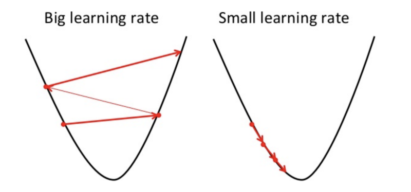
How big the steps are that Gradient Descent takes into the direction of the local minimum are determined by the so-called learning rate. It determines how fast or slow we will move towards the optimal weights. In order for Gradient Descent to reach the local minimum, we have to set the learning rate to an appropriate value, which is neither too low nor too high.

This is because if the steps it takes are too big, it maybe will not reach the local minimum because it just bounces back and forth between the convex function of gradient descent like you can see on the left side of the image below. If you set the learning rate to a very small value, gradient descent will eventually reach the local minimum but it will maybe take too much time like you can see on the right side of the image.

Note

When you’re starting out with gradient descent on a given problem, just simply try 0.001, 0.003, 0.01, 0.03, 0.1, 0.3, 1 etc. as it’s learning rates and look which one performs the best.

8.6. Convergence

Once the agent, after many steps, realize the cost does not improve by a lot and it is stuck very near a particular point (minima), technically this is known as convergence. The value of the parameters at that very last step is known as the ‘best’ set of parameters, and we have a trained model.

8.7. Types of Gradient Descent

Three popular types of Gradient Descent, that mainly differ in the amount of data they use.

8.7.1. Batch Gradient Descent

Also called vanilla gradient descent, calculates the error for each example within the training dataset, but only after all training examples have been evaluated, the model gets updated. This whole process is like a cycle and called a training epoch.

1. Advantages of it are that it’s computational efficient, it produces a stable error gradient and a stable convergence.
2. Batch Gradient Descent has the disadvantage that the stable error gradient can sometimes result in a state of convergence that isn’t the best the model can achieve. It also requires that the entire training dataset is in memory and available to the algorithm.

8.7.2. Stochastic gradient descent (SGD)

In vanilla gradient descent algorithms, we calculate the gradients on each observation one by one; In stochastic gradient descent we can chose the random observations randomly. It is called stochastic because samples are selected randomly (or shuffled) instead of as a single group (as in standard gradient descent) or in the order they appear in the training set. This means that it updates the parameters for each training example, one by one. This can make SGD faster than Batch Gradient Descent, depending on the problem.

1. One advantage is that the frequent updates allow us to have a pretty detailed rate of improvement. The frequent updates are more computationally expensive as the approach of Batch Gradient Descent.
2. The frequency of those updates can also result in noisy gradients, which may cause the error rate to jump around, instead of slowly decreasing.

Stochastic gradient descent

def stocashtic_gradient_descent(X, y, theta, learning_rate=0.01, iterations=100):
   """
   returns the final theta vector and the array of the cost history
   """
   m = len(y)
   cost_history = np.zeros(iterations)

   for it in range(iterations):
      cost = 0.0
      for i in range(m):
         rand_ind = np.random.randint(0,m)
         X_i = X[rand_ind,:].reshape(1, X.shape[1])
         y_i = y[rand_ind].reshape(1,1)
         prediction = np.dot(X_i, theta)

         theta -= (1/m)*learning_rate*(X_i.T.dot((prediction - y_i)))
         cost += calculate_cost(theta, X_i, y_i)
      cost_history[it] = cost

   return theta, cost_history, theta_history

8.7.3. Mini-batch Gradient Descent

Is a combination of the concepts of SGD and Batch Gradient Descent. It simply splits the training dataset into small batches and performs an update for each of these batches. Therefore it creates a balance between the robustness of stochastic gradient descent and the efficiency of batch gradient descent.

1. Common mini-batch sizes range between 50 and 256, but like for any other machine learning techniques, there is no clear rule, because they can vary for different applications. It is the most common type of gradient descent within deep learning.

mini-batch gradient descent

def stocashtic_gradient_descent(X, y, theta, learning_rate=0.01, iterations=100, batch_size=20):
   """
   returns the final theta vector and the array of the cost history
   """
   m = len(y)
   cost_history = np.zeros(iterations)
   n_batches = int(m/batch_size)

   for it in range(iterations):
   cost = 0.0
   indices = np.random.permumtation(m)
   X = X[indices]
   y = y[indices]
   for i in range(0, m, batch_size):
      X_i = X[i:i+batch_size]
      y_i = y[i:i+batch_size]
      X_i = np.c_[np.ones(len(X_i)), X_i]
      prediction = np.dot(X_i, theta)

      theta -= (1/m)*learning_rate*(X_i.T.dot((prediction - y_i)))
      cost += calculate_cost(theta, X_i, y_i)
   cost_history[it] = cost

   return theta, cost_history, theta_history

---

Citations

Footnotes

References

1. Gradient Descent
2. Gradient Descent Linear Regression