3. Example Simple Linear Regression
Different methods used to demonstrate Simple Linear Regression
Ordinary Least Square
- Python from scratch
- Scikit
Gradient Descent
- Python from scratch
- Scikit
3.1. Ordinary Least Sqaure
Creating sample data :
5 6 7 8 | np.random.seed(0)
X = 2.5 * np.random.randn(100) + 1.5
res = 0.5 * np.random.randn(100)
y = 2 + 0.3 * X + res
|
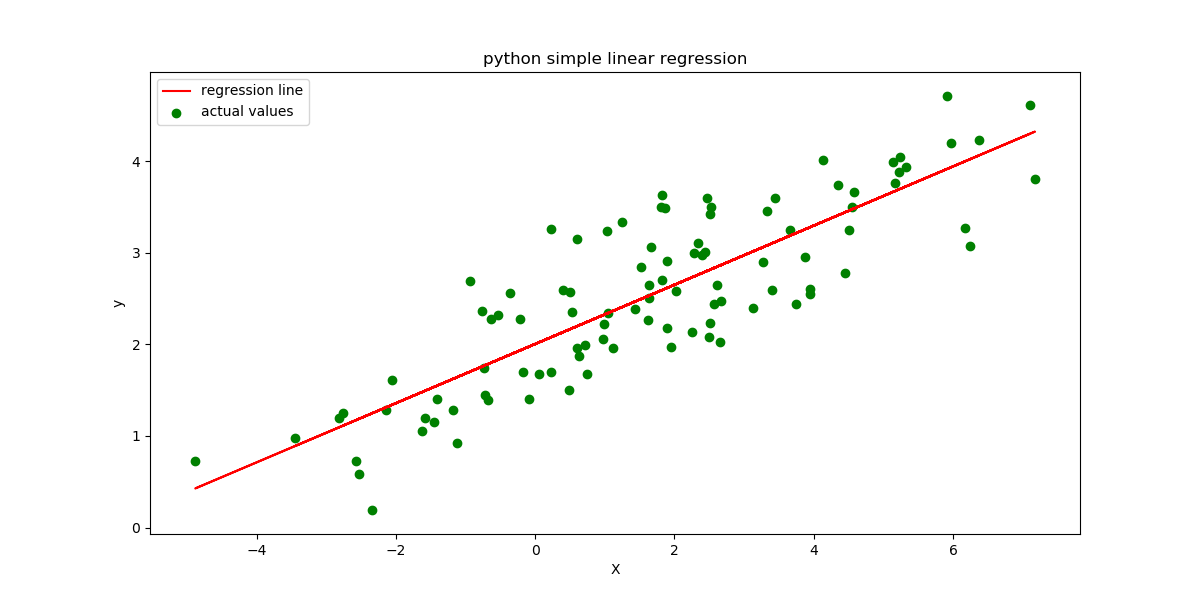
3.1.1. Python
Calculating model coefficiants \(\beta_0\) and \(\beta_1\) :
17 18 19 20 21 22 23 24 | numer = 0
denom = 0
for i in range(100):
numer += (X[i] - mean_x) * (y[i] - mean_y)
denom += (X[i] - mean_x) ** 2
b1 = numer / denom
b0 = mean_y - (b1 * mean_x)
|
intercept: 2.0031670124623426
slope: 0.32293968670927636
Making predictions :
29 | ypred = b0 + b1 * X
|
Plotting the regression line :
32 33 34 | plt.figure(figsize=(12, 6))
plt.plot(X, ypred, color='red', label='regression line') # regression line
plt.scatter(X, y, c='green', label='actual values') # scatter plot showing actual data
|
Calculate the root mean squared error and r \(^2\) error :
37 38 39 40 41 42 43 44 45 46 47 48 49 50 51 52 53 | plt.xlabel('X')
plt.ylabel('y')
plt.legend()
plt.savefig("figure_1.png")
# calculate the error
# root mean squared
rmse = 0
for i in range(100):
y_pred = b0 + b1 * X[i]
rmse += (y[i] - y_pred) ** 2
rmse = np.sqrt(rmse/100)
print("rmse: ", rmse)
# r-squared error
ss_t = 0
ss_r = 0
|
rmse: 0.5140943138643506
r2: 0.7147163547202338
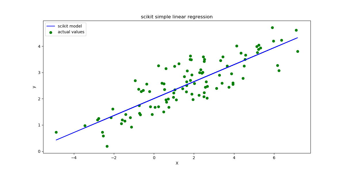
3.1.2. Scikit
Reshape array, scikit cannot use array with rank 1 :
67 | X = X.reshape((100, 1))
|
Initialize model and fit data :
70 71 72 73 | reg = LinearRegression()
# Fitting training data
reg = reg.fit(X, y)
|
intercept  2.003167012462343
slope:  [0.32293969]
Making predictions :
79 | ypred = reg.predict(X)
|
Plotting the regression line :
82 83 84 | plt.clf()
plt.plot(X, ypred, color='blue', label='scikit model')
plt.scatter(X, y, c='green', label='actual values')
|
Calculate the root mean squared error and r \(^2\) error :
92 93 94 95 96 | # Calculating RMSE and R2 Score
mse = mean_squared_error(y, ypred)
rmse = np.sqrt(mse)
r2_score = reg.score(X, y)
print("rmse : ", rmse)
|
rmse :  0.5140943138643504
r2 :  0.7147163547202338
3.2. Gradient Descent
Creating sample data :
16 17 18 19 | np.random.seed(33)
X = 2.5 * np.random.randn(100) + 1.5
res = 0.5 * np.random.randn(100)
Y = 2 + 0.3 * X + res
|
3.2.1. Python
Perform batch gradeint decent with iteration=5000 and learning_rate=0.001 :
35 36 37 38 39 40 41 42 43 44 45 46 47 48 49 50 51 52 53 54 | for i in range(epochs):
# The current predicted value of Y
Y_pred = slope*X + intercpt
# derivative wrt to slope
D_m = (-2/n) * sum(X * (Y - Y_pred))
# derivative wrt intercept
D_c = (-2/n) * sum(Y - Y_pred)
slope = slope - alpha * D_m # Update m
intercpt = intercpt - alpha * D_c # Update c
# reset for next run
D_m = 0
D_c = 0
predictions.append(Y_pred)
intercpts.append(intercpt)
slopes.append(slope)
|
intercept 1.8766343225257833
slope 0.33613290217142805
Calculating the Errors :
69 70 71 72 73 74 75 76 77 78 79 80 81 82 83 84 85 86 87 88 | # root mean squared
rmse = 0
for i in range(100):
y_pred = intercpt + slope * X[i]
rmse += (Y[i] - y_pred) ** 2
rmse = np.sqrt(rmse/100)
# rmse = np.sqrt ( sum ( np.square ( Y - predictions[-1] ) ) ) / 100
print("rmse: ", rmse)
# r-squared error
ss_t = 0
ss_r = 0
for i in range(100):
y_pred = intercpt + slope * X[i]
ss_t += (Y[i] - np.mean(Y)) ** 2
ss_r += (Y[i] - y_pred) ** 2
r2 = 1 - (ss_r/ss_t)
# r2 = 1 - ( sum ( np.square ( Y - np.mean(Y) ) ) / sum ( np.square ( Y - predictions[-1] ) ) )
print("r2 : ", r2)
|
rmse:  0.5135508150299471
r2 :  0.7398913279943503
Plot using matplotlib.animation :
56 57 58 59 60 61 62 63 | ax.scatter(X, Y, label='data points')
line, = ax.plot([], [], 'r-', label='regression line')
plt.xlabel('X')
plt.ylabel('y')
plt.title('python gradient decent')
plt.legend()
anim = FuncAnimation(fig, update, frames=np.arange(0, 5000, 50), interval=120, repeat=False)
anim.save('figure_03.gif', fps=60, writer='imagemagic' )
|
3.2.2. Scikit
Initialize model, default max_iteration=1000 :
100 | clf = SGDRegressor(alpha=alpha)
|
Start training loop. SGDRegressor.partial_fit is used as it sets max_iterations=1 of the model instance as we are already executing it in a
loop. At the moment there is no callback method implemented in scikit to retrieve parameters of the training instance , therefor calling the model
using partial_fit in a for-loop is used :
101 102 103 104 105 106 107 | for counter in range (0,epochs):
# partial fit set max_iter=1 internally
clf.partial_fit(X, Y)
predictions.append(clf.predict(X))
intercpts.append(clf.intercept_)
slopes.append(clf.coef_)
|
intercept 1.877731096750561
slope 0.3349640669632063
Note
Alternatively you could use clf = SGDRegression(max_iter=epochs, alpha=0.001, verbose=1) if you dont want to get the model parameters
during the traing process. verbose=1 enables stdout of the training process.
Calculate the Errors :
112 113 114 115 116 117 | # Calculating RMSE and R2 Score
mse = mean_squared_error(Y, clf.predict(X))
rmse = np.sqrt(mse)
r2_score = clf.score(X, Y)
print("rmse : ", rmse)
print("r2 : ", r2_score)
|
rmse :  0.5135580867991415
r2 :  0.7398839617763866
Plot the training loop using matplotlib.animation :
122 123 124 125 126 127 128 129 | ax.scatter(X, Y, label='data points')
line, = ax.plot([], [], 'r-', label='regression line')
plt.xlabel('X')
plt.ylabel('y')
plt.title('scikit gradient decent')
plt.legend()
anim = FuncAnimation(fig, update, frames=np.arange(0, epochs, 50), interval=120, repeat=False)
anim.save('figure_04.gif', fps=60, writer='imagemagic' )
|
Important
scikits SGDRegressor converges faster than our implementation.
Citations
Footnotes
References